
In the early days of Zcash, I contributed to the first community open source GPU mining implementation Zog Miner. During this work I found a potential (theoretical/mathematical) optimisation that could see decent (reasonably up to 2x) speed increases to the mining algorithms. It turned out, either by design or chance, the Equihash authors prevent this optimisation by limiting the solution space. The logic behind this optimisation is somewhat instructive to understanding the Equihash algorithm, so I've been meaning to write this post ever since I did the initial analysis.
tl;dr - Zcash (and Bitcoin Gold) implement the Equihash algorithm [1] with the constants \(n=200\) and \(k=9\). It is typically assumed that the most efficient list size is \(N=2^{\frac{n}{k+1}+1}\) as the table size doesn't grow per iteration. However, the computation time per solution can be theoretically decreased by increasing \(N\) (which increases the number of solutions) at the obvious cost of extra memory. In practice, implementing this is harder than simply changing a constant in the source of current implementations, as most of the open source projects have been specifically optimized or hard-coded for the \(N=2^{\frac{n}{k+1}+1}\) case. In a mining situation this list size is sub-optimal and can be improved (as we show in this post), however the Equihash paper limits the solution size to \(\frac{n}{k+1}+1\) bits per solution, which limits the solution space and ultimately the list search size to a maximum value of \(N\).
Equihash
Zcash opted for a PoW algorithm that was memory-oriented and ASIC resistant. They ultimately chose Equihash (as has Bitcoin Gold). In a brief chat with Zookoo after Ethereum's Devcon2, he informed me he was aiming for an algorithm that could be run equally efficiently on a CPU as a GPU, leveling the playing field for non-gpu based hardware. As we are all aware now, and as Zookoo knew at the time, the Equihash algorithm falls short of this goal.
The Generalised Birthday Problem
Equihash is an algorithm based on the generalised birthday problem [2]. For those who've not encountered the birthday problem before, it simply relates to the calculation of the probability that in a group of people at least two people have the same birthday. As the wikipedia article demonstrates, the probability of two people in a group of 23 having the same birthday is \(\approx 50\\%\). The probability is non-intuitively high as, although the probability of a singular individual in the group having the same birthday as the others is relatively low, there are many such combinations of group members that can have matching birthdays.
The generalised version of this, aims to find the minimum number of people such that the probability that at least two of them have coinciding birthdays is 50\%.
We will see this kind of problem in action in the Equihash algorithm, however instead of using birthdays we'll be trying to find "matching" hashes. To introduce the algorithm, I'll start with two specific cases, before generalizing to the full Equihash algorithm.
We start by considering two arbitrary 4-bit numbers, \(i_1\) and \(i_2\), along with a hash function \(H\) (which we will use throughout the rest of this post). Our goal is to find two 4-bit numbers such that1,
Solving the above problem is equivalent to solving a 4-bit hash collision, as the XOR of \(A\) and \(B\) will be equal to 0 if and only if \(A = B\). Hopefully the parallel of this example to the singular birthday problem is somewhat clear, in the sense that we are searching through numbers (people) which have matching hashes (birthdays). To further clarify this example, lets look at specific examples. Lets choose \(i_1\) such that \(H(i_1) = 1010\) and \(i_2\) such that \(H(i_2) = 1100\). The preimages \(i_1\) and \(i_2\) are irrelevant for this discussion. We now compute \(H(i_1) \oplus H(i_2)\) which equals \(0110\). As this doesn't satisfy \(\eqref{eq:collision}\) we have not found a solution. However, if we keep \(i_1\) and instead choose \(i_2 \neq i_1\) such that \(H(i_2) = 1010\), the XOR gives \(0000\) and equation \(\eqref{eq:collision}\) is now satisfied. Notice that, in this example, all we've done is produce a hash collision (two different preimages which result with the same hash).
Let us now graduate to a slightly more complicated example. Consider a set of 6, \(10\)-bit numbers, \(i_1 \dots i_6\). The problem we aim to solve is now,
This problem is more indicative of the generalised birthday problem, as we are no longer finding a single hash collision. In this example, we must find 6 numbers (\(i\)'s) such that their hashes XOR to 0.
One naive approach to solve this problem would be to compute the first 5 XOR's and store the result, \(R\). Specifically,
Then permute \(i_6\) until,
which is equivalent to finding a 10-bit hash collision for \(R\). Relating this back to the birthday problem, this is akin to selecting a single person's birthday in a room of many and checking if any of the others have this particular birthday. Drawing from the birthday problem analogy, it is clear that this method is incredibly inefficient as the trick to the birthday problem is that we are not searching for a given individuals birthday to match another's, but rather we are determining if the collective group of birthdays contain a matching pair. Hence there is a faster searching method than this naive case (and it will be discussed shortly).
Let us finally generalize to arbitrary numbers of arbitrary length. Formally, lets consider \(2^k\) numbers of length \(n\) bits, where \(k\) is a natural number. We restrict ourselves here to lists of numbers to be powers of 2 as it aids our analysis in the near future2. The generalized version of equations \(\eqref{eq:collision}\) and \(\eqref{eq:manycollision}\) is,
Although the full Equihash algorithm adds the concept of difficulty, for the time being we will focus on equation \(\eqref{eq:eqhash}\) (ignoring the difficulty filter) to demonstrate how this can be efficiently solved and explain how miner's are currently tackling this problem.
Wagner's Algorithm
Wagner proposed an algorithm for solving this generalised birthday problem efficiently [2]. There are optimisations that can be made to the basic procedure, however we won't go into these in detail as they only distract from the arguments I will present here.
Wagner's basic algorithm is an efficient method for finding a solution to equation \(\eqref{eq:eqhash}\). It is important to note, that the algorithm is designed to solve \(\eqref{eq:eqhash}\) exclusive of the difficulty filter. This is an important point that we will come back to in later sections.
Wagner's algorithm can be summarised by the following procedural steps. Considering a list of \(N\) (this is conventionally set to \(2^{\frac{n}{k+1} + 1}\)) \(n\)-bit numbers, we perform the following steps.
1 - Create a table from the list of numbers (\(X_i\)), that stores the values (\(X_i, i\)). 2 - Sort the table by \(X_i\). Then find all the unordered pairs (\(i,j\)) such that \(i\) and \(j\) are distinct and that \(X_i\) collides with \(X_j\) on the first \(\frac{n}{k+1}\) bits. i.e \(X_i \oplus X_j = 0\) on the first \(\frac{n}{k+1}\) bits. Finally, store the all the tuples (\(X_{i,j} = X_i \oplus X_j, i,j\)) in the table. 3 - Repeat the previous step to find further collisions in \(X_{i,j}\) for the next \(\frac{n}{k+1}\) bits. Store the resulting tuples in the table, i.e (\(X_{i,j,l,m},i,j,l,m\)). This step is repeated until only \(\frac{2n}{k+1}\) bits are non-zero. ... k+1 - The last step involves finding a collision on the last \(\frac{2n}{k+1}\) bits. Any entries left in the table represent solutions to equation \(\eqref{eq:eqhash}\).
Wagner's Algorithm Example
Let us elucidate this algorithm with a clear example. Lets consider \(k=2\) and \(n=3\). In this case, we will create a list of \(N = 2^{\frac{n}{k+1} + 1} = 4\). Lets select (randomly3) the following four 3-bit numbers:
We then sort (\(X_i\)) and create a table of (\(X_i,i\)) like so,
| $X_i$ | $i$ |
| $111$ | 3 |
| $110$ | 2 |
| $101$ | 1 |
| $100$ | 4 |
We now find all the pairs that collide on the first \(\frac{n}{k+1} = 1\) bit. Notice in our case, this is all the entries. We therefore find the permutations that collide, specifically, (\(3,2\)), (\(3,1\)), (\(3,4\)), (\(2,1\)),(\(2,4\)) and (\(1,4\)). We proceed by storing the \(X_{i,j}\) colliding tuples with their indexes in a new table sorted by \(X_{i,j}\) , like so,
| ${X_{i,j}}$ | $(i,j)$ |
| $011$ | (2,1) |
| $011$ | (3,4) |
| $010$ | (2,4) |
| $010$ | (3,1) |
| $001$ | (3,2) |
| $001$ | (1,4) |
Typically this procedure would be repeated multiple times. However given the small \(k\) and \(n\) we are now ready to check the final \(\frac{2n}{k+1}=2\) bits. Doing so, we can see that the only tuple containing unique indexes is (\(1,2,3,4\)) (recalling that order doesn't matter as the XOR operation is commutative).
Thus we arrive at our solution that:
and hence if the \(X\)'s we started with correspond to the hashes of some numbers, i.e \(X_j = H(i_j)\) then the \(i_j\)'s would represent the solutions to \(\eqref{eq:eqhash}\).
Analysis of Wagner's Algorithm
Lets explore some simple analysis of the time complexity and memory requirements of performing Wagner's algorithm. To do so, we assume that sorting a list of size \(L\) can be done in \(O(N)\) which is computationally equivalent to \(L\) calls to the hash function \(H\). In what follows we set a single call to the hash function \(H\) to be our time unit.
Expected Number of Solutions
Although the example above gave a list which contained a solution, it is possible that lists contains no solutions. The larger the list size, the greater the chance of it containing many solutions, but also the greater the computation time and memory usage to process and store the list. Also note that the list size from one collision search to the next is statistical in nature, there is no certainty that it doesn't grow or shrink from one iteration to the next. Wagner's algorithm is designed such that on average, the list size remains approximately constant between collision searches and that approximately only 2 solutions are found. Again, remember, it was designed to solve equation \(\eqref{eq:eqhash}\) and not to find many solutions (which may be optimal for mining purposes, which we explore later when we introduce the concept of difficulty). Lets explore this result that there are 2 solutions on average found with Wagner's algorithm.
The key to minimizing computation time to find a single solution to equation \(\eqref{eq:eqhash}\) comes by setting the list to size \(N = 2^{\frac{n}{k+1} +1}\). We expect the bits of the elements making up the list to be uniformly distributed (they are chosen randomly) so that after the first collision search, we expect (i.e. the average) there to be
entries in the second table. Note that we don't store duplicate entries, i.e. \((1,2)\) is equivalent to \((2,1)\). To understand the derivation of equation \(\eqref{eq:firstcol}\), note that we don't expect all entries in a randomly populated list to collide on the first \(\frac{n}{k+1}\) bits. In fact for a single bit of a given singular entry there is a 50\% (or \(\frac{1}{2}\)) chance that another entry has the same bit (the entry can be either 0 or 1 with equal probability). Thus, the probability that two entries will collide on the first \(\frac{n}{k+1}\) bits is simply \((\frac{1}{2})^{\frac{n}{k+1}} = \frac{2}{N}\). The expected table length is given by the number of possible distinct permutations of two items, chosen from the original list of N items (namely \({}^NC_2=N(N-1)/2\)), multiplied by the probability that the first \(n/(k+1)\) bits of a given pair collide (namely \((\frac{1}{2})^{\frac{n}{k+1}})\), which gives equation \(\eqref{eq:firstcol}\).
Now that we know the length of the second table, we can calculate the expected length of the third table by replacing \(N\) on the left-hand side of equation \(\eqref{eq:firstcol}\) with the value \(N-1\). This gives
where \(\langle T_L^{(2)} \rangle\) denotes the expected table length after \(2\) iterations. We see that, on average, the third table is expected to contain \(O(N)\) entries for \(N\gg1\). This iterative process can be repeated to derive a general expression for the expected table length after \(m\) iterations:
In particular, after \(k-1\) iterations, only \(\frac{2n}{k+1}\) bits remain uncollided and the expected table length is \(N-2^{k-1}-1\). We determine the expected number of solutions by checking for collisions on the final \(\frac{2n}{k+1}\) bits. The probability that two entries collide on all remaining bits is \(2^{-\frac{2n}{k+1}} = (\frac{2}{N})^2\), while the number of pairs to test is
Combining these gives the expected number of solutions4:
where the last approximation is valid when \(N\gg 2^k\), which is equivalent to \(k \ll n/(k+1)\).
We can check the accuracy of the above approximation by using the general expression for \(\langle S \rangle\) to estimate the expected (average) number of solutions for zcash, i.e. \(n=200, k=5\). In this case, the expected number of solutions per run is
consistent with the approximation \(\langle S \rangle \approx2\), which is often used in the literature.
In summary, we have demonstrated that Wagner's algorithm generates an average of 2 solutions to the hashing problem, per run, and the expected table length is approximately constant for large \(N\).
Computation Complexity and Memory Requirements
In what follows, we restrict ourselves to the assumption that \(N \gg 2^k\) (N is much larger than \(2^k\)), in which case we can safely assume that the list size remains constant throughout the search process.
The computation complexity is governed by the list generation and subsequent sorting of each list throughout each step. The list generation requires \(N\) calls to the hash function and there are \(k\) sortings of N. Accounting for the initial list generation, the total time complexity is
The memory usage is obtained by calculating the number of bytes we need to store in order to maintain the lists in each iteration. Let's briefly explore this in general. Initially, the first list is of size \(N\) and consists of numbers of \(n\) bits. There are therefore \(nN\) bits in this list. However, the first table we construct consists of \(X_i\) as well as \(i\) itself, which is a number that must be able to represent every element in \(N\). If \(N\) is of size \(2^{\frac{n}{k+1}+1}\) then \(i\) itself must be at least a \(\frac{n}{k+1}+1\) bit number. Assuming that the size of the list remains constant after each collision search, the index's \(i\)'s double; i.e. we start with a single index, then after a collision, we have a pair of indexes \((i,j)\), then after a further collision we have four indexes \((i,j,l,m)\) and so on. Thus by the last iteration, we need to store a table that contains the tuples (which will be of bit size \(2^{k-1}( \frac{n}{k+1} + 1)\), where the \(2^{k-1}\) comes from the doubling of the indexes) and all the XOR'd elements, each of size \(n\) bits. Ultimately we require the following memory in bytes:
Here we have multiplied by \(N\) as there are \(N\) elements in the final table and divided by \(8\) to convert from bits to bytes.
Ok, so this is all well and good, but what is the point of all this, you may ask. Well, the above analysis becomes important once we introduce the notion of difficulty and ask a rather fundamental question, simply, is this list size the best for solving a block with the Equihash algorithm?
Difficulty
In order for a Proof of Work (PoW) system to function, we typically introduce the concept of difficulty. Difficulty is simply a filter or threshold that we apply to solutions of algorithms before we accept them as valid solutions. This allows tuning of the amount of work miners need to perform in order to solve blocks (in a blockchain context). In the Equihash case, to include difficulty and apply this algorithm to a blockchain setting, we modify our fundamental problem (given by equation \(\eqref{eq:eqhash}\)) slightly.
We take some seed variable, denoted \(I\) (which is derived from the block header, see [3] for further details) and a nonce, \(V\), and modify the original problem stipulated in \(\eqref{eq:eqhash}\) to5:
The difficulty filter is also added, whereby the protocol only accepts solutions such that:
Here \(d\) is some number that represents how difficult it is to find a solution. The main difference between \(\eqref{eq:eqhash}\) and \(\eqref{eq:difficulty}\) is that \(\eqref{eq:difficulty}\) includes a nonce, \(V\), such that it is now possible to find many solutions, simply by permuting the nonce. The idea is that, once a solution to \(\eqref{eq:difficulty}\) is found, it is checked to see if it passes the difficulty filter, if it does not, the nonce is incremented (or randomized) and the algorithm runs again.
Potential Improvements
If we recap slightly, we see that Wagner has found an efficient method for finding on average, two solutions given a list of size \(N = 2^{\frac{n}{k+1}+1}\). Wagner did not consider algorithms that would produce a large number of solutions, as why would anyone want a large number of solutions to a given problem, especially if it is more computationally expensive.
However, now that we have introduced the difficulty filter, if we apply Wagner's algorithm, we get 2 solutions (on average), we check those solutions against the difficulty and if they do not pass, we repeat Wagner's algorithm. It therefore seems reasonable to ask the question, what is more efficient, running Wagner's algorithm to find 2 solutions and repeating, or modifying the algorithm to find many solutions in one go?
This problem is based on the fact that we are no longer trying to find an algorithm that optimises a singular solution to the generalised birthday problem, but we are now trying to optimise an algorithm which finds a solution to a block (which necessarily requires passing a difficulty filter). Thus, it may be computationally beneficial to search for multiple solutions in order to have a greater probability of passing the difficulty than to simply find 2 solutions and repeat the entire algorithm. Ultimately, we are posing the question: Is solving many solutions in one pass cheaper than solving the same number of solutions in many passes? In order to answer this question, we will use some of the analysis we completed in the previous sections.
General Premise
So far, I've left out some important details about the Equihash algorithm, specifically some constraints which stipulate that Wagner's algorithm must be used to find solutions6. Thus, we cannot modify the core procedure of Wagner's algorithm listed here, to find more solutions, we can only modify some of the variables used in the algorithm. In this case, we are going to explore the list size \(N\). The conventional list size of \(N = 2^{\frac{n}{k+1}+1}\) is used because on average, the list size remains constant through each collision search and it also provides 2 solutions, as we have seen in our previous analysis. If we were to decrease \(N\), then the list size would shrink at each iteration and we would statistically find less solutions each pass. If we increase \(N\), the list size should grow each iteration, but we would also find more solutions. The goal here is to find out whether it is optimal to increase the list size, in order to find more solutions per run to increase our chance of solving a block. There will inevitably be a time/memory trade off as the greater we increase the list size, the more memory we will consume. Anyway, let's do some math and find out.
Expected Number of Solutions
Lets explore the available parameter space for Wagner's algorithm by generalizing the relationship between \(N\), \(n\) and \(k\). That is, we will no longer demand that \(N=2^{\frac{n}{k+1}+1}\) and will instead allow \(N\) to be arbitrary. In particular we will be interested in larger list sizes as we expect to find more solutions.
We start as we did in the Wagner case, by estimating the table size throughout each collision iteration. As we found in equation \(\eqref{eq:firstcol}\), after the first collision the average table size is:
We have assumed \(N \gg 2^1\) in the last step, to simplify the expression. This result is identical to \(\eqref{eq:firstcol}\) with the exception that terms have not been simplified by assuming \(N=2^{\frac{n}{k+1}+1}\).
If we repeat the collision process \((k-1)\) times (by iteratively replacing the resulting \(N\) as the initial list size to be collided) we should obtain the table size
We can finally estimate the expected number of solutions from this, as only \(\frac{2n}{k+1}\) bits remain uncollided. Colliding these final bits gives the expected number of solutions, per algorithm run:
Equation \(\eqref{eq:g:sols}\) gives us the expected number of solutions for arbitrary initial list size \(N\). We can now estimate, how much time and memory is required in order to obtain these solutions. These will become important in determining whether this method is indeed faster when it comes to solving blocks.
Time Complexity and Memory Requirements
An arbitrary list size, is of course going to effect our time complexity and memory requirements. Lets start by estimating the amount of memory (naively) we would need for an arbitrary list of size \(N\).
The memory can be estimated from the list size of the last table, i.e \(\eqref{eq:g:listsize}\). For each element in the list, we need to store the \(n\) bit numbers and the \(2^{k-1}\) tuples each of \(\lceil \log_2 N \rceil\) bits. The \(\log_2 N\) is just the number of bits required to store the index for a tuple. The resulting memory requirement (which is an over-estimation as more efficient algorithms can be used) becomes:
We can plot this memory requirement (\(M\)) relative to the Wagner case (\(M_W\)) as a function of initial list size, \(N\). This is shown in the figure below.
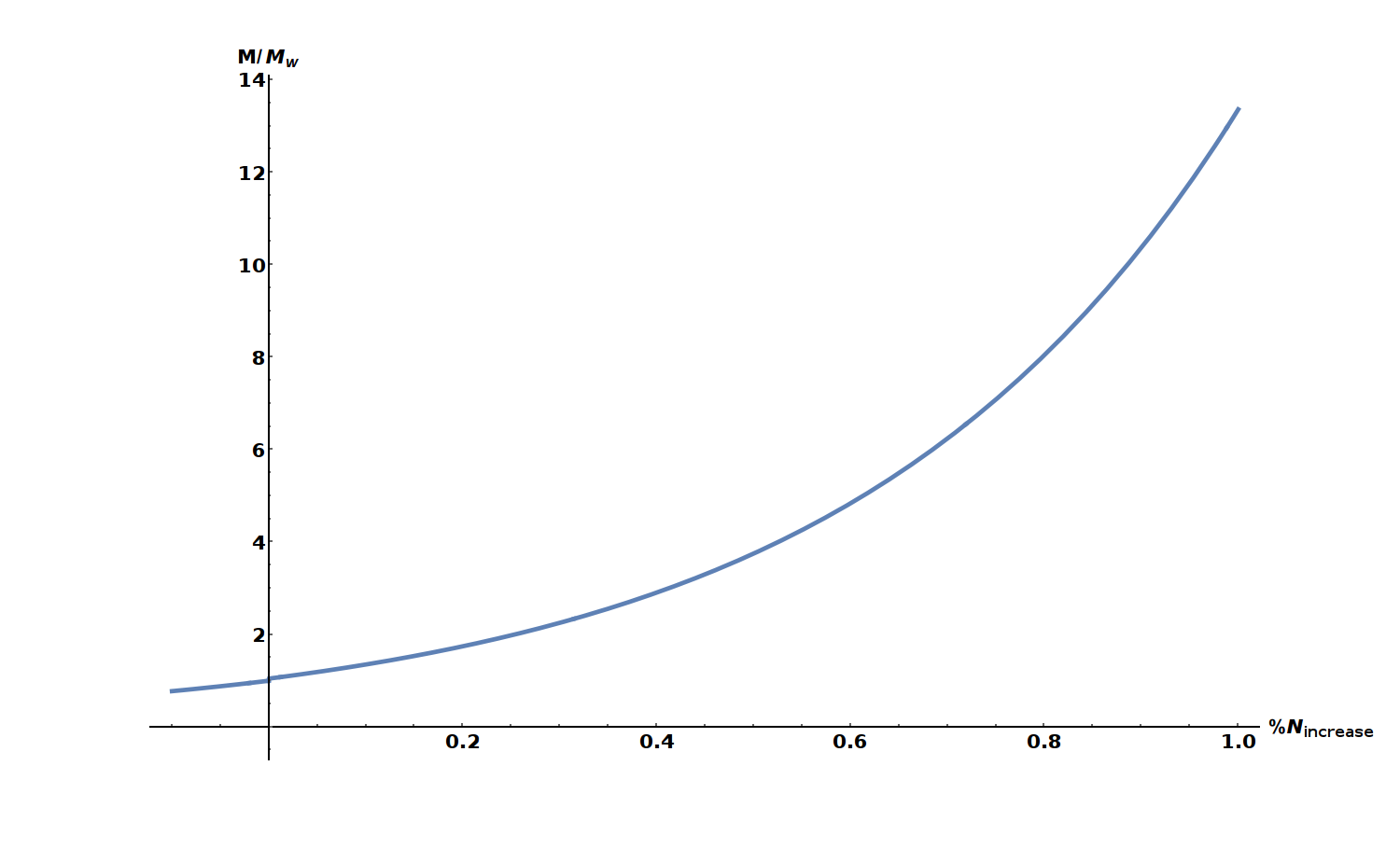
The x-axis shows the increase in list size compared to Wagner as a percentage. We see that a 1% increase in list size requires about 14x more memory to run the algorithm.
The above result is somewhat expected, obviously a greater list size will require more memory. The interesting part, will be estimating algorithm time complexity for arbitrary list sizes.
Generating the initial list requires \(N\) calls to the hash function, while sorting a list of length \(N\) involves a time complexity equivalent to N calls of the hash function (as we calculated in the Wagner case). The generalised version thus is simply,
where we've set the table length after 0 collisions to the initial list length,i.e \(\langle T_L^{(0)} \rangle \equiv N\).
We can now finally calculate if increasing the list size is optimal in PoW scenarios. The final missing ingredient is applying the difficulty filter.
Satisfying the Difficulty Constraint
Recall that in order to find a valid solution in the Equihash algorithm, we require the solutions we find to pass a difficulty filter. From our previous discussion, we know that the difficulty \(d\) is simply an integer that specifies the number of 0's required for our solution to be valid (see \(\eqref{eq:difficulty:d}\)).
Now, the probability that a given solution \(S\) will have \(d\) leading zeros is simply \((1/2)^d\). If the algorithm generates \(\langle S \rangle\) average solutions to the hashing problem, per run, the average number of solutions per run that satisfy the difficulty constraint will be \(\langle S \rangle \times 2^{-d}\). Thus, the average number of times the algorithm must be run, in order to generate a solution that satisfies the difficulty, is
Therefore, the average time complexity required to obtain a solution to a block is
This finally gives us the time complexity for solving a block of difficulty, \(d\). We can plot this time complexity (\(T\)), relative to the time complexity of using Wagner's list size (\(T_W\)) for percentage increases in the list Wagner list size.
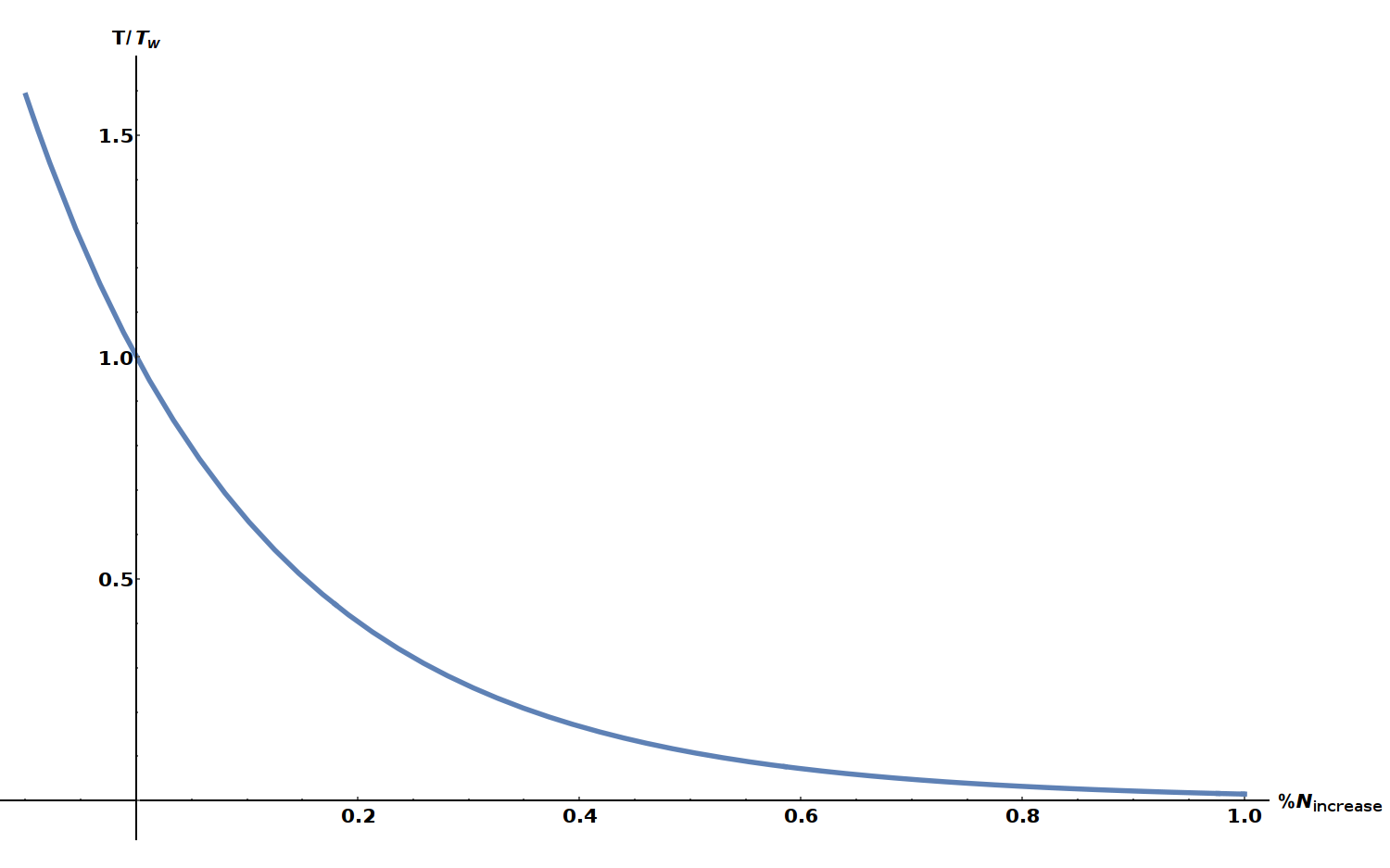
The above plot is independent of difficulty (it is canceled in the ratio). It is clear that there are significant time-complexity reductions simply by increasing the list size. In fact, we see about a 98% speed increase if the initial list size is increased by a single percent. We should also keep in mind that this increases also requires a 14x increase in memory to achieve the speed reductions.
There is a small caveat to this result, which is applicable only for small difficulties. In equation \(\eqref{eq:algruns}\) when estimating the number of algorithm runs required to solve a block, we've allowed non-integer values for the algorithm run. If, on average, it requires 1.2 algorithm runs to solve a block, often we we will have to run the algorithm twice in order to see a solution. This is exemplified in the case when the difficulty is really low, let's say \(d=1\), then on average it will take 1 algorithm run to solve a block (assuming we use Wagner's list size and obtain 2 solutions on average, see \(\eqref{eq:algruns}\)). Then, if we were to increase the list size, we would obtain more solutions, let's say on average 100, and our average number of algorithm runs, would be mathematically equivalent to 1/50. We can't half run the algorithm, so we would have to run it once (which would cost more time than the Wagner's solution, due to the larger list sizes) obtain 100 solutions and solve a block. This would be more computationally expensive than running Wagner's algorithm, for this low difficulty.
We can approximate this effect by taking the ceiling of the expected number of algorithm runs, when estimating the time complexity. i.e
The time complexity to solve a block is then dependent on the difficulty when compared to the standard Wagner list size. If we plot this for a few values of difficulty, \(d\) we can see that this method is less efficient in some cases for lower difficulties. However as the difficulty increases gains we see approach that which we found when ignoring the fractional algorithm runs (shown in our previous figure).
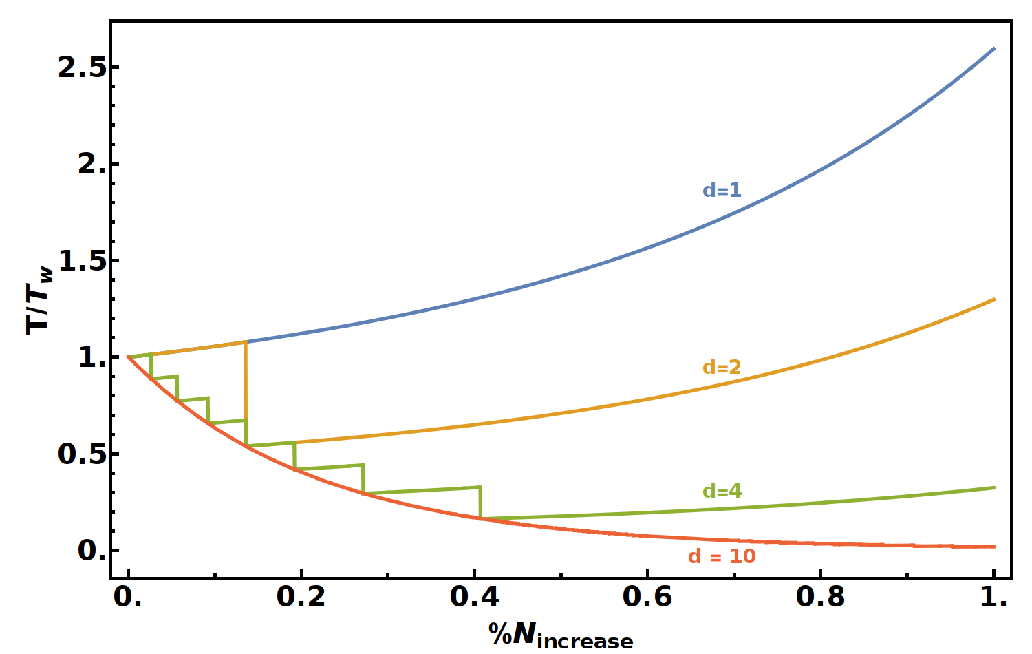
It is clear that for small difficulties there is no gains to be made, but as the difficulty increases, the time complexity gains approach our previous estimates. If one were to build a solving algorithm for small difficulties, the list size should be dependant on the difficulty such that it is chosen to produce on average an integer number of algorithm runs. This is associated to the steep drops in the above graph, signifying dramatic optimisations at that particular list size.
Finally, it is important to clarify that these optimisations come with a memory trade off. We can gain time reductions at the cost of memory increase. To demonstrate this clearly, I've made a log plot of the memory and time reductions.
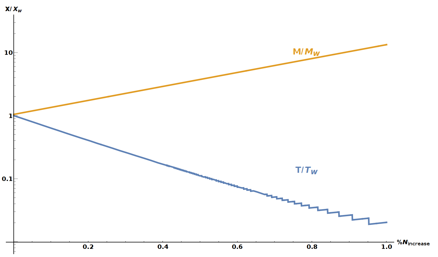
This was plotted with \(d=10\), which still shows some step-like fluctuations due to non-integer average algorithm runs. Fundamentally, this analysis allows us to choose an time efficiency given our appetite for increased memory usage.
Application to Equihash
Everything described in this blog is general with respect to the generalised birthday problem and Wagner's algorithm to solving the problem. There is an issue with directly applying the above optimisations to the equihash algorithm however. The Equihash paper [1] describes the algorithm as we described here, with one vital detail. They specify the input solutions, (the values to be entered into the hash, in our notation \(i_k\)) to be \(\frac{n}{k+1} +1\)-bit numbers. This is the exact bit length of Wagner's table size. Thus, if we increase the table size at all, we would require a larger bit-length to represent the extra solutions. Although these solutions could solve the conditions in \(\eqref{eq:difficulty}\) and \(\eqref{eq:difficulty:d}\), they would be rejected by implementation that impose this condition. By limiting the bit size of the pre-images, the algorithm binds itself to solution space of only Wagner's \(N\) number of solutions, fundamentally rendering this optimisation useless.
For those interested in applying this to Zcash or bitcoin gold, both implementations currently limit the solution-space per nonce to Wagner's \(N\) :(.
Conclusion
Although potentially futile, we have looked over the Equihash PoW algorithm in depth and explored potential optimisations to block-solving software. In particular, increasing the initial list size, we could see speed improvements of over 65%, at the cost of over a 14x increase in memory. This analysis showed that the algorithm has a clear time/memory trade-off should any implementation of equihash not require the \(\frac{n}{k+1} +1\)-bit length of the solutions.
In any case, hopefully this post was somewhat informative as to how Equihash works.
References
[1] - A. Biryukov and D. Khovratovich, Equihash: Asymmetric Proof-of-Work Based on the Generalized Birthday Problem, 2015, e-print.
[2] - D. Wagner, A Generalized Birthday Problem, 2002, DOI:10.1007/3-540-45708-9_19.
[3] - D. Hopwood, S Bowe, T. Hornby and N. Wilcox, Zcash Protocol Specification, 2017, Online PDF.
-
For those unfamiliar with the XOR operator (\(\oplus\)), it is an operation that takes the individual bits of each object it acts on, say, A and B, and returns true if A or B is one (true) but not both. ↩
-
Wagner's algorithm will be introduced and analysed with respect to list numbers that are powers of 2, however, this algorithm does generalise to arbitrary positive list sizes. ↩
-
This example was far from random, chosen carefully to demonstrate the algorithm. In practice, random numbers are used. ↩
-
In this equation we approximately equate this to \(2\) under the assumption that \(N >> k\). ↩
-
The symbol \(||\) refers to concatenation. ↩
-
This is enforced by ensuring that intermediary bits of the solution hashes collide, which is a signature property of Wagner's algorithm. You can see this occurring in the tables where I gave a simplistic example. See [1] for further details. ↩